Meteorology of the February 25, 2004
Flash Flood Event at San Francisco State University
Updated 3/11/04
Images: Courtesy of Dept of Geosciences Weather Graphics and Simulation Lab, University of Wyoming and the U. S. Navy
Note: The analyses contained herein are entirely the conception of John Monteverdi. The contents of this page do not necessarily reflect the opinion of anyone else connected with the Department of Geosciences and/or San Francisco State University. While questions regarding the analyses are welcomed, individuals wishing additional analyses, opinions or the raw data should contact primary sources or seek the services of a consulting meteorologist. Except where otherwise noted (one exception, noted below), copying of images is allowed, as long as attribution is made to the Department of Geosciences.
- General Overview
- Rainfall Estimates
- Radar View of Storm and Sounding/Hodograph Analysis
- Satellite and Map Views of Storm
A. General Overview
San Francisco State University, southwestern San Francisco County and northwestern San Mateo County experienced a torrential rain storm associated with a convective cell that passed over the area between 8:30AM and 9AM on 25 February 2004.
The rainfall was the most intense I have ever seen at San Francisco State since I have been here (1979). A rain gage in the City of San Francisco's Department of Public Works network is sited on the roof of our building (Thornton Hall). That gage recorded 1.90" in the 45 minutes ending at 9AM (at which time the power went out), 1.56" in 30 minutes. This is an extraordinary rainfall intensity*, and more is said about it in the next section.
*Note: As of 3/11/04, I and representatives of the SFPUC have surveyed the SFSU gage twice since the 25 February storm. The system consists of (a) a Qualimetrics tipping bucket rain gage (part of the SFPUC rain gage network); (b) a Teloger data logger; and, (c) software to process the data from (a) and (b). All facets of the system were surveyed in June 2003 (as they are on a yearly basis), with the system calibration checked at that time, with everything given a clean bill of health. We have disassembled the rain gage housing and already have decided that the rain gage itself is fine. SFPUC representatives are checking the data logger and software. As of this time, it appears that the five minute intensities were accurate, but that the clock times were offset systematically (adjusted for human observations of peak rainfall below). Until all systems are given a clean bill of health, the rainfall totals from SFSU's rain gage should be viewed with some caution.
The resulting flooding was awesome. 19th Avenue had water estimated by a chemistry colleague of mine to be 4 feet deep, which then spilled over the sidewalks and down to the play field adjacent to this building. The cascades down that 15 foot section were reminiscent of pictures you see of waterfall/cascades in tropical rain forests.
All the streets around Thornton Hall were flooded to about 2 to 3 feet. Students reported that Lake Merced Blvd had 4 feet of standing water, 19th Avenue through Golden Gate Park was so flooded that cars were up to their hoods and stranded.
B. Rainfall Estimates
The flooding was not related to the 24 hour rainfall amounts that occurred in the Bay Area from the storm of of 2/25/04. These were large, but not particularly remarkable, as shown in the figure which follows.

This map above was constructed using totals from the National Weather Service and the San Francisco Chronicle. It is an estimate and should not be considered "official" in any sense of the word. Most areas of the northern and central Bay Area received between 1.5" to 5" for the 24 hour period ending Midnight 2/26/04. But the flooding was related to the high intensity rainfall that occurred in the morning of 2/25/04.
The chart below shows rainfall intensities by 5 minute periods for San Francisco State University, and four other locations in southern San Francisco County. The high intensities were capped by a 5 minute total of 0.42" for the five minute period ending 8:55AM at San Francisco State University. The table beneath the chart shows the same data in tabular form, also including several other stations for which 5 minute data in San Francisco was available.

| Ending Time/2-25 |
SF State* |
Lake Merced |
Sun. HS |
1680 Miss |
Miss. Ed |
| 8:10 |
0.01 |
0.01 |
0.02 |
0.01 |
0.01 |
| 8:15 |
0.03 |
0 |
0.03 |
0.02 |
0.01 |
| 8:20 |
0.06 |
0.01 |
0.03 |
0.02 |
0.02 |
| 8:25 |
0.25 |
0.02 |
0.02 |
0.03 |
0.03 |
| 8:30 |
0.18 |
0.03 |
0.04 |
0.03 |
0.02 |
| 8:35 |
0.24 |
0.14 |
0.18 |
0.32 |
0.25 |
| 8:40 |
0.35 |
0.06 |
0.20 |
0.09 |
0.22 |
| 8:45 |
0.17 |
0.12 |
0.15 |
0.07 |
0.17 |
| 8:50 |
0.20 |
0.09 |
0.15 |
0.21 |
0.28 |
| 8:55 |
0.42 |
0.09 |
0.08 |
0.20 |
0.27 |
| 9:00 |
0 |
0.20 |
0.02 |
0.12 |
0.05 |
| 9:05 |
0 |
0.13 |
0.03 |
0.05 |
0.02 |
| Peak 15 min |
0.79 |
0.42 |
0.53 |
0.53 |
0.72 |
| Peak 30 min |
1.56 |
0.69 |
0.80 |
1.01 |
1.24 |
Note: Rainfall Information Courtesy of Ron Hundenski, San Francisco Public Utilities Commission (All data preliminary. Use SFSU information with caution. Gage is being checked).
Using the totals shown in the table above, and other information kindly provided by Dr. Ron Hundenski of the SF Public Utilities Commission (SFPUC), the return periods for the peak 30 minute totals from fifteen gages in the SFPUC were determined and plotted on the chart below. Please note that four of the nineteen gages in San Francisco County were not reporting, including three in extreme south-central California, so interpretation of the contours in that area should be made with caution. In addition, the last contour drawn was for the 1000-year 30-minute rainfall event. The shaded area is the estimate for the portion of the map experiencing the 10000-yr 30-minute rainfall event, but since that is based solely on the information from the gage at SFSU, we are awaiting final determination on the status of that gage before plotting that contour.
The map above should not be interpreted too closely. The return period isopleths were drawn based upon the information from only fifteen gages in San Francisco county. The pattern shown is consistent with the radar evidence, which shows a very intense convective cell moving across the region, first over northwestern San Mateo County into San Francisco, as explained below. We fully expect the data we are able to obtain from places in Daly City to show a similar pattern. In short, the isopleth pattern is consistent with the movement of the radar echo, as described below, and it can be assumed reliably that at least a 1000 yr rainfall event (for 30 minutes) moved across the southwestern 1/3 of San Francisco County and, inferentially, across the northwestern portion of San Mateo County.
Concept of Return Period
Use the return period information with great caution. The concept of return period is often misused. In order for return period information to be somewhat useful and valid for meteorological information at least a 30-year sample of information should be obtained. That is because only for a 30-year or longer period of record for rainfall information will the statistics calculated for that sample be somewhat representative of the same statistics calculated for the longer record, if it existed. As an example, there is about a 64% probablity that a 30-yr record will actually contain a true 30 yr storm (as a storm is defined, for any duration). There is only a 26% probability that a 30-yr record will actually encompass the 100 yr storm (from Bruce and Clark, 1966, p. 130).
Even if the return periods could be interpreted in a straightforward manner, the term 100 yr storm does not mean that such an event would only occur once in a century, but that over a very long period, say 500 years, such a storm would occur 5 times, on average. In essence, there is a 1% chance that such an event would occur in any given year. Even so, such a concept is grounded in the assumption that climate has not changed.
Thus, the terms "1000 y" or "10000 yr" event, as appear in the table above, are statistical artifacts; they appear in the statistics, but really have little DIRECT meaning, because of the shortness of the record. However, such terms do establish the relative severity of the event, and can be used to establish that (a) an event is extreme; and, (b) the relative (as opposed to absolute) infrequency of the event is established statistically; and (c) the event was unusual and not to be expected typically in a lifetime.
Bruce, J.P., and R. H. Clark, 1966: Introduction to Hydrometeorology. Pergamon Press. 319 pp.
|
Also, when the cell moved to Oakland, it passed nearly over my house, which does have a recording rain gage, measuring intensities by 30 minute intervals. This is shown below. About 1 inch of rainfall occurred there between 9:30AM and 10:30AM, with lots of local flooding in Oakland too.

© Property of John Monteverdi. Use is authorized for display only.
There has been much in the news in which the flooding was attributed entirely due to backed up culverts and drainage systems, perhaps improperly cleaned. Although the role of culverts and drainage systems in any possible flooding should be studied by engineers rather than be a source of speculation, the fact of the matter is that it would be very unusual for any drainage system to be able to handle such enormous rainfall rates, which are probably on the upper end of what we can expect in the lowland areas of the Bay Region for 1/2 hour. Such rainfall rates as were observed with this storm are typical of flash flood producing thunderstorms in other portions of the country and are very atypical for the Bay Area.
C. Radar View of Storm and Sounding/Hodograph Analysis
The cell embedded in the main area of moderate rain was clearly depicted by KMUX WSR-88D National Weather Service radar in the Santa Cruz Mountains. The radar plot for 8:27AM PST 2/25/04 is shown below.
Base Reflectivity -- 1/2 Degree Tilt--KMUX 17:02 UTC
(Image from WGSL, courtesy of Dave Dempsey, edited by John Monteverdi)
The radar shows a small, elongated area of convection, oriented from southwest to northeast, along the back edge of the front. These were cumulonimbus clouds that had a length of about 10 miles but a width of only abourt 2 to 3 miles. One passed over Daly City and southwestern San Francisco, eventually getting to Oakland and Berkeley, but largely missing the northwestern 1/3 of San Francisco.
In this image, the radar captured the leading edge of the heaviest rainfall (indicated in orange and red), corresponding to rainfall rates on the order of 1 1/2 to 2 1/2 inches per hour. The motion of the radar echo was such that, fortunately, it only remained over any one area for 20 to 30 minutes. Even so, rainfall of 0.75" to 1.50" occurred in that 20 to 30 minute period.
The sounding reproduced below is that of KOAK at 12 UTC, a time at which the Bay Area was just on the leading edge of the frontal band. I have superimposed the sounding on the back edge of the frontal band to show the destabilization (consistent with the cumulonimbus development) that took place in the lower troposphere (note: the portion of sounding in the upper middle and upper troposphere and the dew point profile below 900 mb were substantially the same as that at 12 UTC). The thermodynamic conditions on the rear portion of the frontal band supported penetrative convection.

Interestingly, the hodograph at 12 UTC (characeristic of the wind profile until the frontal band passed, after the flood event), favors supercellular convection. We are trying to get velocity images from KMUX to place here as well, because, anecdotally, we have found out that the convective cell was rotating, and associated with a waterspout just southwest of San Francisco.
The hodograph shows a pronounced veer of the wind shear vector with height from the surface to 850 mb, combined with deep layer shear of around 5.0 X 10⁻³ s -1. In plain English, both of these measure the degree to which the manner in which the wind directions and speeds change with height support rotating updrafts in the thunderstorms that may have developed that morning.
D. Satellite and Map Views of the Storm
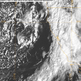
The visible satellie shown below captures the back edge of the storm as it was moving across north-central California (Image: Courtesy of U.S. Navy).
1745 UTC Visible Satellite --Note Convective Elements Evident in Texturing over Northern California
Texturing (a three-dimensional look to the cloud on this image suggesting convective towers casting shadows on the lower overcast) evident in the frontal band is evidence of cumulonimbus growth in scattered areas.

Zoom of 1745 UTC Visible Satellite Image
Note the shadowing showing the southwest-northeast orientation of the convective cells shown in this close up zoom of the same image. I have pointed out several of them. The northern-most one corresponds to the cell that shows up well on the radar plot above.
1645 UTC IR -- Note infrared "texturing" on the north side of frontal band passing through Bay Area. Other convective signatures clearly evident off the south-central California coastline, and in the large area of cellular cloudiness off the Northern California coastline. (Image produced by Dave Dempsey)
MORE TO COME
Summary: Meteorological Overview Photo Pages: Page 1 | Page 2 |
John Monteverdi / montever@sfsu.edu / revised
3/11/04/